Managing product descriptions with Oracle Enterprise Data Quality
Many organisations purchase the same products from multiple suppliers and commonly ask the suppliers to provide data as to the manufacturer, description, part number etc. Unfortunately each supplier usually has their own format for the data they supply and no way to convert the content into a format specified or required by the buyer. Oracle Enterprise Data Quality provides a range of tools and techniques for dealing with the issues resulting from this Babel of data and this document outlines one of the common variants in which the only information provided is a part id and the product description field.
The description field
The description field in these situations has no standard format. It is an assortment of similar sorts of information, in the examples below including units of measure, types of product, colours, dimensions, materials, product name etc. The order of these elements can be random and the representation of the same value between two rows can be different, for example STEEL and STL.
Examples of typical values:
1 1/8-12X4 HX HD CAP SCR-GR 8 ZINC PL(LE)
1/2-13X4 1/2 HX HD FULL THRD CAP SCR GR 2
The target system at the client requires structured data records. Therefore the attribute data such as size, material, head type etc must be extracted, duplicates detected and managed, and individual records for each item produced.
The challenge is to understand the data, match it, and restructure it as follows:
| Original Description |
Base Description |
Category |
Head Type |
Material |
Screw Type |
Dimensions |
Grade |
| 1 1/8-12X4 HX HD CAP SCR-GR 8 ZINC PL(LE) |
HEX HEAD CAP SCREW- ZINC PL(LE) |
SCREW |
HEX HEAD |
ZINC PLATED |
CAP |
1 1/8-12X4 |
GR 8 |
| 1/2-13X4 1/2 HX HD FULL THRD CAP SCR GR 2 |
HEX HEAD FULL THRD CAP SCREW |
SCREW |
HEX HEAD |
|
CAP |
1/2-13X4 1/2 |
GR 2 |
To achieve this, we use EDQ to:
- Profile the description field to understand the contents
- Classify each record to the high level categories e.g. SCREW, BOLT, HAMMER etc
- Identify key pieces of information in the data
- Extract these attributes into appropriate fields
- De-duplicate the extracted records
- Format the output according to the requirements of the target system.
The sample data used in this document has been curated to include a number of didactic data points and is broadly similar to data encountered in real customer scenarios.
Profiling
Profiling is a simple but essential stage when working with a new source of data, be it a text file, Excel spreadsheet, XML or JSON file or database table. Data sources often contain odd values, manifestly erroneous values, historical data overloading to get round application restrictions, duplication etc., and empty cells where we would expect to find real data. EDQ’s profiling tools give you a quick, simple but focused set of analysis tools.
Here we have a simple EDQ process which uses 4 of the available EDQ profilers. This process works from left to right. The first processor, labelled “Sample Product Data Input”, is a Reader which gets data from wherever it is sourced and then routes it to the activity processors.
Quickstats processor
The Quickstats profiler is a quick, general purpose profiler which displays 5 metrics on each of the select columns, in this case there are only 2 columns, ‘Id’ and ‘Original Description’
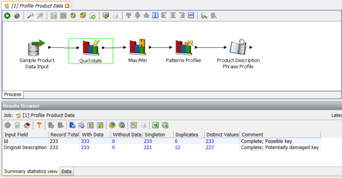
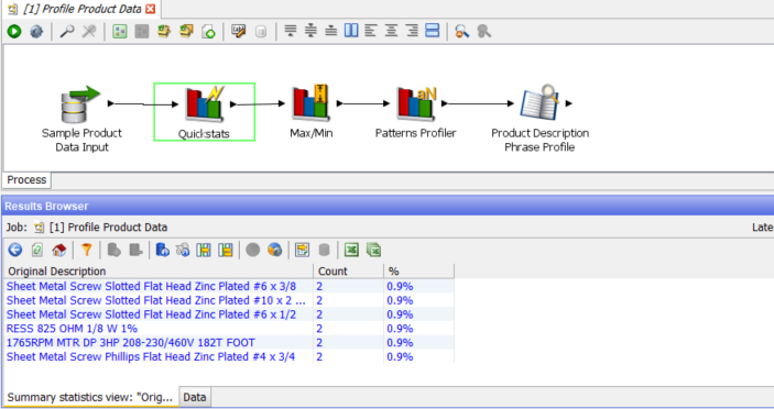
The blue cells in the Results Browser indicate cells where we can drill down into the raw data. In this case most of the results are as expected. All cells are populated and the only anomaly is the 12 Duplicates in the ‘Original Description’ column. Drilling in to the blue 12 we see there are 6 values which are each duplicated once for a total of 12 rows:
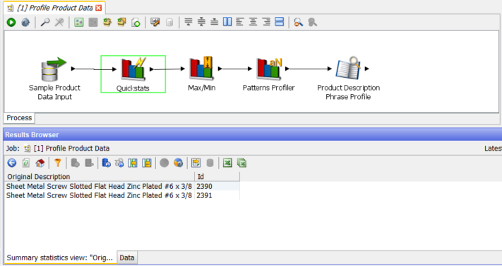
Drilling down further into one of these we find that although the original description is the same, the ‘Id’ number is different. This should be noted for further investigation.
Max/Min processor
Sometimes a processor doesn’t reveal any anomalies and simply confirms that in a particular dimension the data is in good shape:
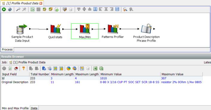
Here we would not expect to learn much useful about ‘Original Description’, but for ‘Id’ we do see that the numbers are in the range of three and four digits and the distribution is not over an extreme range.
Patterns Profiler
The results for this profiler show much more variety:
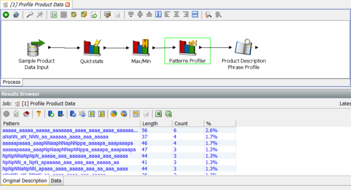
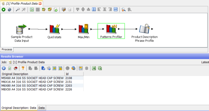
The most common pattern only occurs 6 time (out of 233 rows) and there is a lot of variation in the patterns. Drilling in to the second row we find:
Looking at a number of the other patterns it is clear that the data contains rows relating to several different types of product. There are many screws, but also bolts, capacitors, motors and resistors. And it is also clear that for each type of product there are many different patterns. This means that the job of extracting the information we need will require care. If, for example, we knew that all of the records related to screws, and that the second word from the right always contained the head type, then it would be relatively simple to design a process to extract this information. However, it is clear that the data contains several types of product (not just screws), and that the key information that we need to extract is often presented in a different order, often for the same type of product.
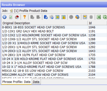
Phrase Profiler
The Phrase Profiler is one of the more configurable profilers. It tokenises the input string, by default on strings but it can use any delimiters, into the constituent tokens which it the profiles on frequency. The example here is a simple single token configuration but it is also often useful to combine tokens into phrases, for example to detect ‘cross head’ for screws whenever is occurs.
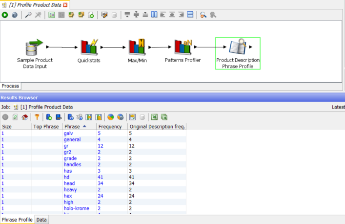
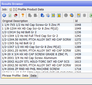
Note that ‘gr’, ‘gr2’ and ‘grade’ reveal on drill down the same effective value – ‘grade’. The example of ‘hd’ and ‘head’ covers 75 rows:
These results will be used in standardisation and extraction to populate the attributes appropriately:
-
The data contains rows relating to several different types of product:
o Screws
o Bolts
o Capacitors
o Motors
o Resistors
- The description field contains many different patterns. The important information that we will need to extract is presented in different orders. Our extraction process must cater for this. In other words, it must include semantic, as well as pattern-based recognition capabilities.
- The data contains different abbreviations of the same value (screw and scr). Our process will need to first recognize these as meaning the same thing and then standardize them.
Classification
We will now use a different process to perform the initial categorisation and classification. This is done for clarity – we could have added the following steps on to the original process.
The first job we need to perform on product descriptions is to classify each row into its primary category. If we can identify a row as being for some variant of, for example, screw then we narrow down the steps required to identify and extract all of attributes which apply to screws, without having to worry about looking for any attributes which would apply to a motor.
The reader in this process reads the exact same two columns of data as the reader in the previous process. At the top right we have a new processor type, the Writer, which writes data out to the staged data stores within the EDQ repository. If we look at the data in the Writer we will see that we have an additional column:
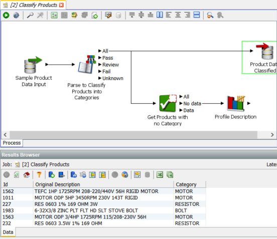
The Category column has been filled with a category value derived from the data in ‘Original Description’. This data has been derived by the Parse process which is one of the most powerful processors in EDQ:
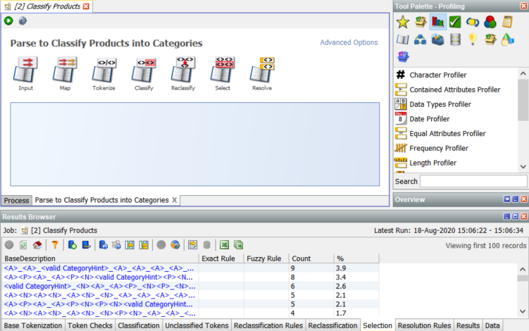
The Parser has 7 dialogs which control its configuration. For the purposes of this document we will only look at the Classify dialog:
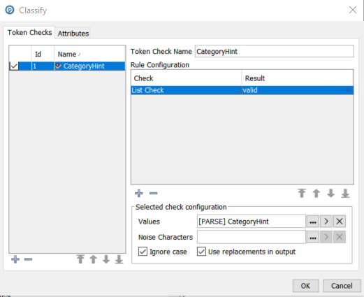
This configuration says that we will perform a list check using the individual tokens in the ‘Product Description’ column and that will use the values in the resource table ‘[PARSE] CategoryHint’. Note the checkbox ‘Use replacements in output’ – this will result in the derived ‘Category’ being output. The ‘[PARSE] CategoryHint’ contains the following:
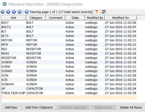
You can see here that we have multiple synonyms for bolts, motors, resistors, screws and capacitors which will be replaced by the value in the Category column in the reference data. If the processor find a token equal to ‘SCREW’, ‘SCRW’, ‘SCRWS’, ‘SCW’, ‘SCR’ or ‘SCREWS’ then it will assign the row to the ‘SCREW’ category. EDQ ships with sets of pre-prepared reference data, and the reference data can be extended with data from the Phase Profiler and can also be created from scratch, either with the EDQ Director interface or in e.g. Excel which can later be inserted or imported into reference data.
Extracting Dimensions
In this section we will go through a more sophisticated analysis of the ‘Product Description’ column and extract the dimensions of the screws in the data. This section is performed as a walkthrough adding to an incomplete process:
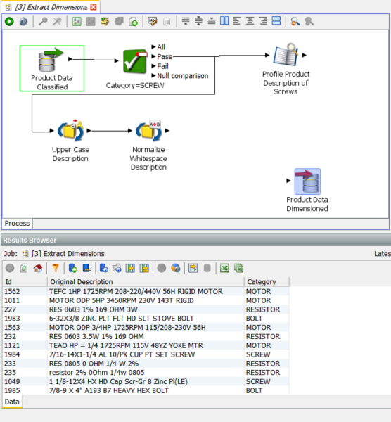
We have now changed the reader definition and are using the output from the previous process with the added ‘Category’ column.
The next processor is a simple value check to split the data into the ‘SCREW’ category and to ignore everything else. The configuration of the value check is:
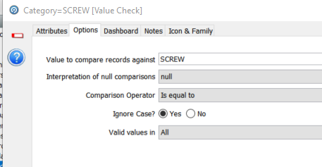
Each value in ‘Category’ is compared to the value ‘SCREW’. If true then the row is passed on. If not then it is, in this case, ignored.
The first processor is a Phrase Processor which we originally saw in the basic profiling section. The configuration of this instance is richer, in particular for multi token phrases:
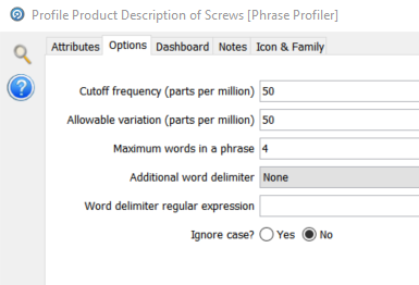
The maximum words in a phrase is now set to 4. This means that any continuous set of one to four tokens will be included in the frequency count:
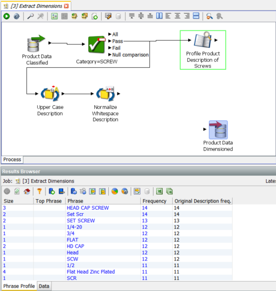
We now get multi token phrases like ‘SET SCREW’, ‘HEAD CAP SCREW’ and ‘Flat Head Zinc Plated’
The ‘SCREW’ data stream is also forked to the processor ‘Upper Case Description’ followed by ‘Normalize Whitespace Description’. These are simple standardisations, the former changes the case of all letters to upper case and the latter removes spaces from the beginning of strings and compresses all multiple space sequences into single spaces.
Adding the first ‘Extract Attribute’ processor
The Extract Attribute processor looks for specific patterns in the description fields which are data for specific attributes of the category we are examining, in this case ‘SCREWS’.
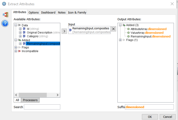
Configuring the processor:
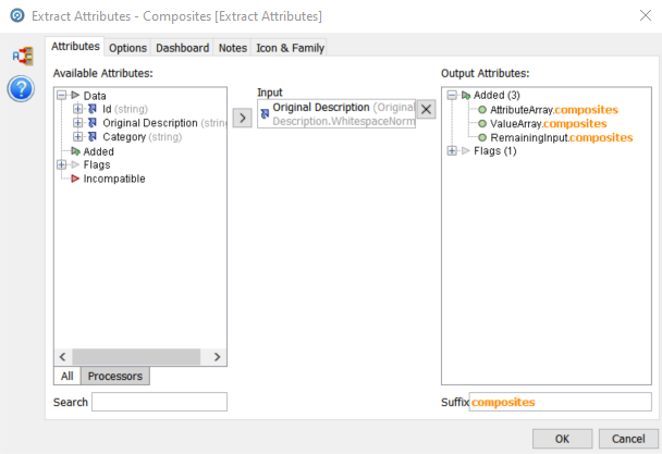
First we configure the input column, in this case ‘Original Description’. The output attributes by default are always ‘AttributeArray, ValueArray and RemainingInput. We have added the suffix ‘composites’ to indicate that it can include a number of attributes as we will see.
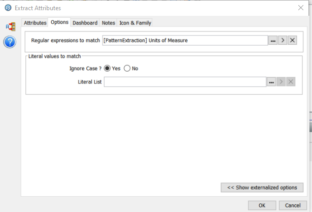
We then select the ‘Options’ tab and configure the resources required:
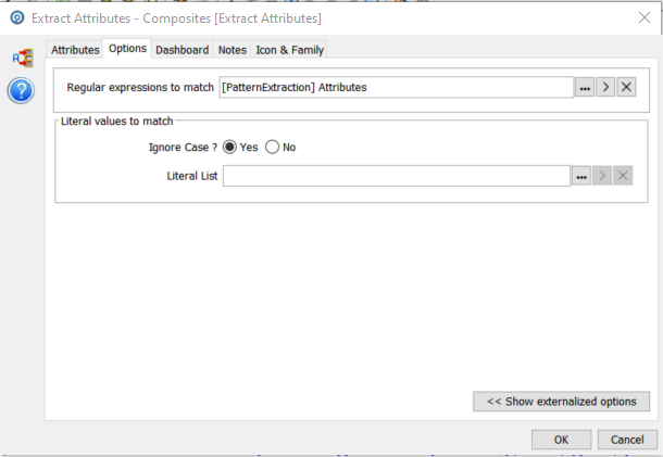
The ‘Extract Attributes’ processor is driven by regular expressions. We will cover the details of this after viewing the output.
We can also specify Literal values if we are working, for example with name-value pairs. This does not apply in this case.
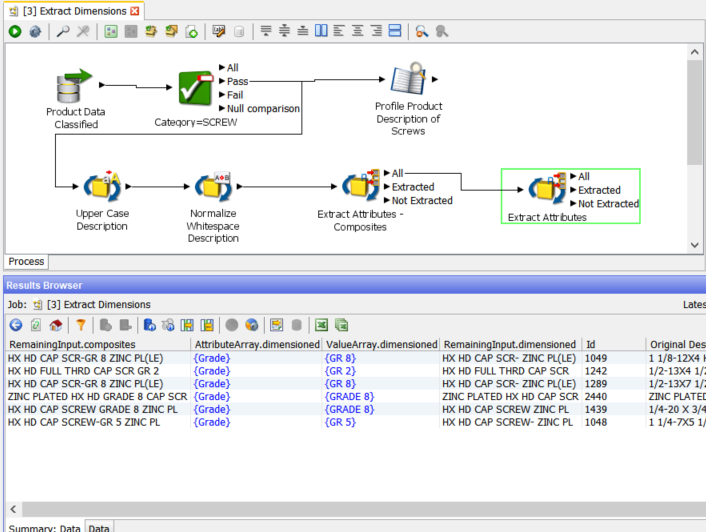
We now run the process and then examine the Results Browser for the ‘Extract Attributes – Composites’ processor:
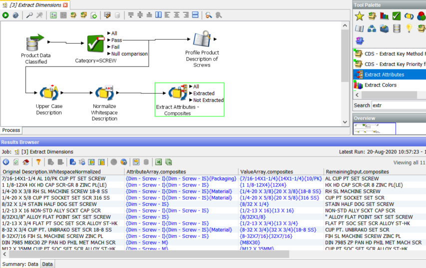
We have the three new columns, ‘AttributeArray.composites’, ‘ValueArray.composites’ and ‘RemainingInput.composites’.
Looking at the first row we see that ‘AttributeArray.composites’ contains an array of three values, {Dim – Screw – I}{Dim – Screw – IS}{Packaging}, which are the names of the three found attributes, two dimensions and one packaging.
The values for these attributes are contained in ‘ValueArray.composites’, {7/16-14X1-1/4}{14X1-1/4}{10/PK}. The first one, ‘Dim – Screw – I’, is the complete dimensions of the screw while the second, ‘Dim – Screw – IS, is a short form. The ‘Extract Attributes’ processor supports nested attribute definitions. The final attribute ‘Packaging’ is a simple 10/PK, i.e. 10 pack.
The reference data driving this processor is a regular expression table which allows us to simply but precisely define the patterns which represent attribute data:
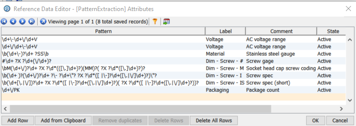
The last new column is ‘RemainingInput.composites’ which contains ‘AL CUP PT SET SCREW’ i.e. what remains after extracting the attributes. The processor extracts pieces of information that are important to us and placed them in new attributes. Meanwhile, with some of the ‘noise’ of dimensions removed, the stripped back description field is now easier to understand, and so it is easier to extract more information from it. To use an analogy, we have peeled back the first layer of the onion. This is often useful as input to a follow on ‘Extract Attributes’ processor or for review of outliers.
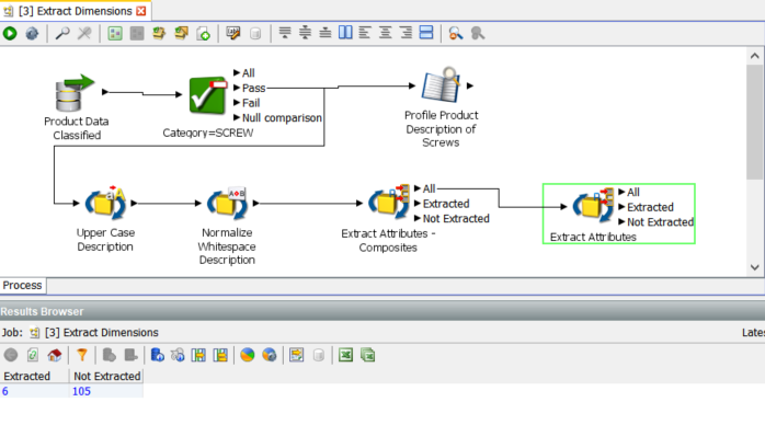
The second Extract Attributes processor
We configure the second ‘Extract Attribute’ processor to use the ‘RemainingInput.composites’ columns, as described above, with a suffix of ‘dimensioned’ as we are going to extract units of measure this time:
With a different set of regular expressions to extract units of measure:
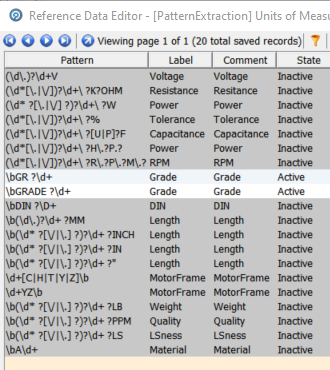
This illustrates another useful feature of the reference data mechanism. It is possible to use one list but change the State of individual rows between Active and Inactive. In this case we have chosen to only extract the ‘Grade’ attribute.
With such a restricted set of ‘Active’ rows in the reference data we get a limited set of extractions, in this case, 6:
Drilling down:
Preparing for output
We now have two pairs of arrays, one for the composites and one for the grades. To make this useful we will need to persist it. We cannot write arrays directly to a database or text file so we need to normalise this representation. We also need to discover what format our end user requires, and for the purposes of this document we are going to assume that the required format is name-value pairs for each attribute in a single concatenated text field, as this allow us to demonstrate a range of tools and techniques.
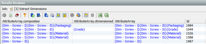
Concatenating the Attribute and Value arrays
This is simple using the ‘Concatenate Arrays’ processor which takes two (or more) arrays in sequence and creates one array with all elements. We need to do this twice in this case, once for Attributes and once for Values:

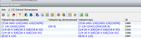
The screen shot shows the configuration for the Values array. We take the two arrays as the Selected Attributes and name the output “ValueArrays” with no suffix.
The results for Attributes:
The results for Values:
Normalising the arrays
A common output requirement is one row per name-value pair, so if a row has 3 element arrays, we generate 3 rows for one input record, 2 for 2, 1 for 1 etc.
The ‘Split Records from Array’ processor does this:
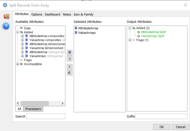
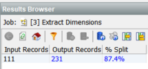
The result metrics:
The result data:
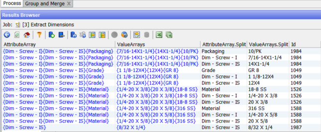
Note the multiple rows per Id.
Creating the name-value pairs
To achieve this we use a simple ‘Concatenate’ processor. In the previous step we generate the split single entry version of both the attributes and their values. Now we want to concatenate the ‘AttributeArray.Split’ and ‘ValueArray.Split’ values using a delimiter of our choice into the default output field for the ‘Concatenate’ processor, ‘concat’:
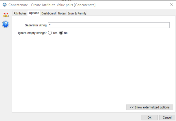
We have used the carat as the delimiter as there are spaces and dashes in the data.
Combining the Name-Value pairs for each Id
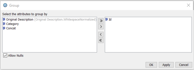
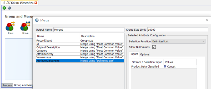
The ‘Group and Merge’ processor performs this function. It will group all records on the Id column, and merge all fields apart from ‘Concat’ (the name-value pairs value) on the basis of most common value as all the values will be the same. The ‘Concat’ field will use the ‘Delimited List’ selection function to create a single string of all of the ‘Concat’ name-value pairs for the same ‘Id’, delimited by a character of our choice.
We define the group attribute:
And then we define the selection function for ‘concat’ and name the output ‘NameValuePairs’:
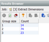
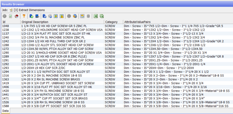
The summary results show that we are back to 111 rows:
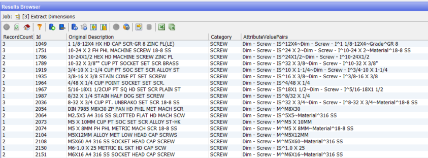
And we can see in the merged data that we have a single string with 1, 2 or 3 constituent attribute-value pairs with distinct delimiters:
Write out the data
There is a second, follow on blog to this one which will cover two advanced features, parsing and matching. We need to store the results so far into the EDQ repository so it can be picked up by the next process.
The EDQ repository has a results schema which can be used to store data for inter process and inter job persistence. The ‘Writer’ processor takes the working data from a process and writes it out to a staging table:
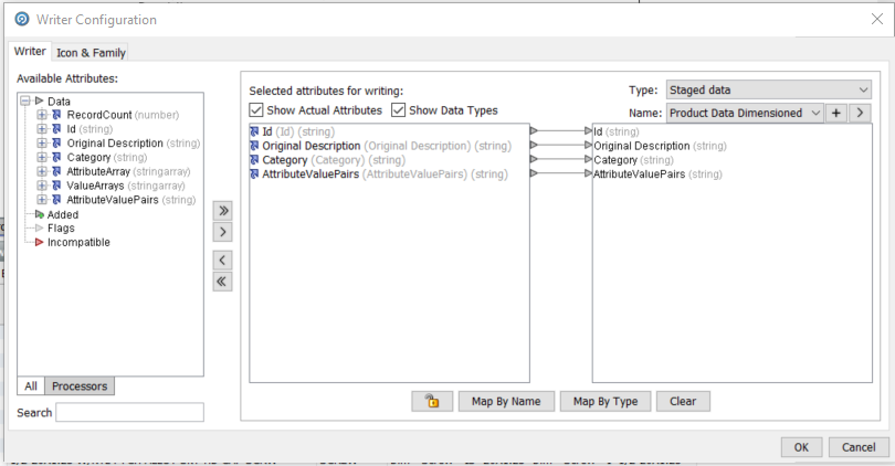
We have selected the most important fields and only persisted that data:
Summary
This walk through illustrates some of the variety of techniques and tools available in EDQ for managing product data, specifically to do with classification and attribute identification and extraction.
The second half covers the use of parsing to standardise data and matching to identify duplicates and also to check for detail changes over time.
This post is based Mike Matthews’ <mike.matthews@oracle.com> Oracle OpenWorld Hands On Lab.