Extending SaaS by AI/ML – Part 3: Text classification without Training Dataset

Introduction

This marks the third installment in our blog series titled ‘Expanding SaaS with AI/ML Capabilities.’ If you haven’t had a chance yet, you can explore our previous blogs below. Up to this point, we’ve covered topics such as extracting data from SaaS through BICC extracts and object storage, as well as setting up a notebook session and installing a Conda environment within OCI Data Science. The Jupyter Notebook is utilized for the purpose of developing a machine learning model tasked with categorizing items into distinct item classes. 

Part 1: Using SaaS Data
Part 2: Model data preparation using OCI Data Science

This setup is ideal when we have a training dataset to construct and subsequently deploy a production-ready model capable of classifying real-time items into distinct item classes. However, what if we encounter a scenario where a training dataset is unavailable, yet we still require a mechanism for item classification? In such cases, relying solely on static rules for classification can quickly become complex, especially when dealing with highly unstructured data that varies from one customer to another. This blog explores the approach of using machine learning to classify items even in the absence of a training dataset. 

Before we discuss on the actual solution, it’s essential to discuss key concepts related to Text Embeddings and Cosine Similarity.

Text Embeddings

Text embedding is a technique used in natural language processing (NLP) and machine learning to convert text data, such as words, sentences, or documents, into numerical vectors. These numeric representations empower various tasks including text summarization, document retrieval, and document classification. Multiple techniques exist for generating sentence embeddings, such as the Sentence Transformer (Hugging Face) and the Cohere Embedding APIs. We will discuss more about Cohere Embedding APIs in this blog. The reference section also contains links that offer additional information.

Cosine Similarity

Cosine similarity is a measure used in machine learning and natural language processing (NLP) to determine the similarity between two vectors (text embeddings), Cosine similarity ranges from -1 (perfectly opposite) to 1 (perfectly identical), with 0 indicating orthogonality (no similarity). The reference section also contains links that offer additional information.

Use Case: Classify Item Description into distinct Item Classes without any training dataset

Architecture

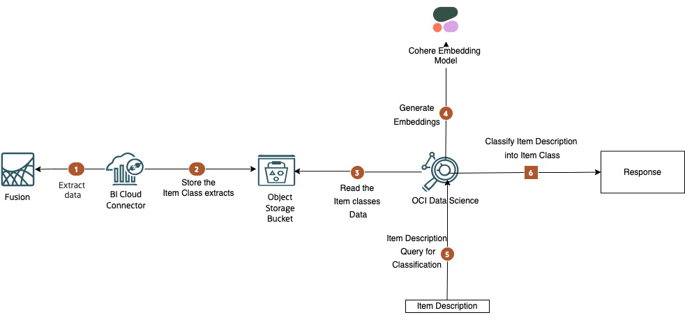
This solution demonstrates a method for classifying item descriptions without relying on a training dataset, utilizing embeddings and cosine similarity. The concept behind this approach is to employ it as an initial solution in situations where there is no existing training data. As more data is collected through human/customer feedback, the intention is to subsequently train a Supervised Classification model for improved accuracy.

Steps

• Step 1: Within the Fusion environment, a BICC job is employed to extract the item classes defined in the Fusion Product Data Hub and compile them into a compressed CSV zip file.
• Step 2: Subsequently, this zip file is uploaded to Object Storage for storage and accessibility.
• Step 3: OCI Data Science retrieves the zip file from Object Storage and proceeds to decompress its contents.
• Step 4: Utilizing the Cohere Embedding API, the item classes undergo a transformation process into vector embeddings.
• Step 5: The Item Description query is also converted into an embedding. Following this, a cosine similarity calculation is initiated between the item description and the embedding of item classes.
• Step 6: Drawing upon the cosine similarity data, the item class that exhibits the highest degree of similarity to the query is returned as the top recommendation. Furthermore, reranking algorithms can be employed to further refine the results and enhance their quality.

Illustration

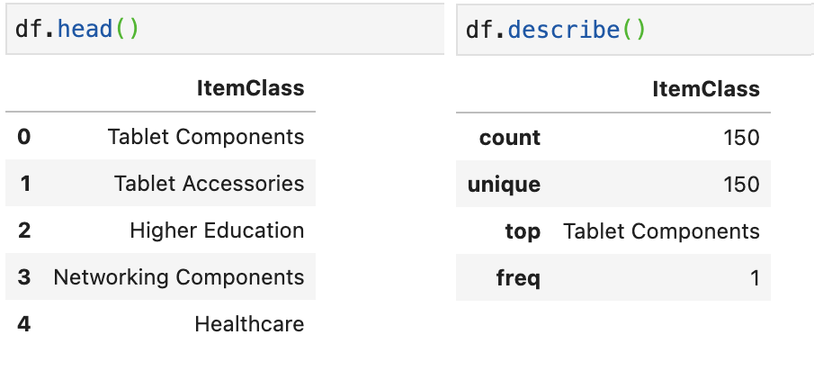
The item class CSV file undergoes conversion into a Pandas DataFrame, and below, you’ll find the first 5 records among the 150 unique item classes.

Next, we initiate the process of generating embeddings for Item Classes through the Cohere Embedding APIs. You have the flexibility to select any suitable model for embedding generation.

# Generating the embeddings for Item Classes
ItemClassList = df['ItemClass'].tolist()
embeddings = co.embed(model='embed-english-light-v2.0',texts=ItemClassArray).embeddings
f"embeddings vector size : {len(embeddings[0])}"

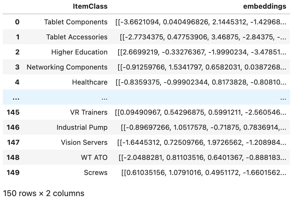
The cohere model embedding vector size is 1024. These embeddings are then transformed and added to the existing Pandas DataFrame, introducing two columns: ‘itemclass’ and ’embeddings.’

# Transforming & adding embeddings to DataFrame
df['embeddings'] = embeddings
def transform_embeddings(item):
    item['embeddings']=[item['embeddings']]
    return item

df = df.apply(transform_embeddings,axis=1)
df

Finally, we proceed to generate the embedding for Item Descriptions and perform a cosine similarity comparison with the embeddings of item classes. As a result, the top recommendation for item classification is returned.

# Run cosine similarity bewteen Item Description and Item Classess
item_description = 'Bodum Assam Teapot'
item_desc_embeddings = co.embed(model='embed-english-light-v2.0',texts=[item_description]).embeddings
def cosine_score(item):
    item['cosine_score']=cosine_similarity(item['embeddings'],item_desc_embeddings)[0][0]
    return item
df = df.apply(cosine_score,axis=1)
item_class = df.loc[df['cosine_score'].idxmax()]['ItemClass']
print("'{0}' is classified as '{1}'".format(item_description,item_class))

Large Language Models

Large Language Models (LLMs) have significantly streamline the classification process. LLMs can provide real-time classification of text data, making them suitable for applications that require quick decision-making.

Prompt Base Approach: LLMs can categorize the item using the provided item description. This can be achieved by supplying an appropriate prompt along with the item description and list of item classes. It’s important to note that each LLM has a context window that restricts the number of tokens the model can process as input when generating responses. This approach is particularly effective when the entire prompt fits within the context window.

Retrieval Augmented Generation: The RAG approach becomes particularly valuable when the list of item classes exceeds the context window limit of the LLM, and you still require the LLM to classify item descriptions. To implement this, the item classes must first be converted into embeddings and stored in a Vector DB or Open Search with an ANN Plugin.

When using the RAG approach, the same prompt can be provided to the LLM, but without including the item class list. The LLM will then reference the Vector DB to retrieve the top relevant item classes through a similarity search with the item description. It will then utilize these top-ranked item classes to classify the item description into the intended item category. The upcoming blog will discuss this scenario in greater detail. Please stay tuned for more information.

Fine Tuning: When there is an ample amount of training data available for item classification, as discussed in part-2 of the blog, it becomes feasible to fine-tune LLMs using a specialized training dataset containing item descriptions and their corresponding item classes. This fine-tuning process combines the broader knowledge from a pre-trained model with task-specific data, ultimately enhancing the model’s performance in item classification.

References

• https://blogs.oracle.com/ai-and-datascience/post/introduction-to-embedding-in-natural-language-processing
• https://txt.cohere.com/sentence-word-embeddings/
• https://docs.cohere.com/docs/similarity-between-words-and-sentences